Nowcasting revisions using the generalized Kishor-Koenig family

This vignette describes the generalized Kishor-Koenig (KK) revision model and its nested variants as implemented in reviser::kk_nowcast(). The exposition uses the same Durbin-Koopman state-space notation that appears throughout the package documentation: observation matrices are denoted by $Z$ , transition matrices by $T$ , shock-loading matrices by $R$ , and disturbance covariance matrices by $H$ and $Q$ (Durbin and Koopman 2012).

The motivation is straightforward. Early releases of macroeconomic series are often revised several times before they settle near a stable value. Rather than ignoring that revision process, the KK family models the vector of releases directly and uses the Kalman filter to infer the latent efficient estimate.

Revision system

Suppose that an efficient estimate becomes available after $e$ revisions. Let $y_t^j$ denote the $j$ -th release for reference period $t$ , where $j = 0, \dots, e$ . Following Strohsal and Wolf (2020), stack the efficient estimates and the observed real-time releases as

$z_t = \begin{bmatrix} y_{t-e}^{e} \\ y_{t-e+1}^{e} \\ \vdots \\ y_t^{e} \end{bmatrix}, \qquad y_t = \begin{bmatrix} y_{t-e}^{e} \\ y_{t-e+1}^{e-1} \\ \vdots \\ y_t^{0} \end{bmatrix}.$

The generalized KK model is

$z_t = F z_{t-1} + \nu_t, \qquad \nu_t \sim N(0, V),$

$y_t = (I - G) F y_{t-1} + G z_t + \epsilon_t, \qquad \epsilon_t \sim N(0, W).$

The companion-form transition matrix is

$F = \begin{bmatrix} 0 & 1 & 0 & \cdots & 0 \\ 0 & 0 & 1 & \cdots & 0 \\ \vdots & \vdots & \vdots & \ddots & \vdots \\ 0 & 0 & 0 & \cdots & 1 \\ 0 & 0 & 0 & \cdots & F_0 \end{bmatrix},$

and the gain matrix is

$G = \begin{bmatrix} 1 & 0 & \cdots & 0 \\ G_{e-1,e} & G_{e-1,e-1} & \cdots & G_{e-1,0} \\ G_{e-2,e} & G_{e-2,e-1} & \cdots & G_{e-2,0} \\ \vdots & \vdots & \ddots & \vdots \\ G_{0,e} & G_{0,e-1} & \cdots & G_{0,0} \end{bmatrix}.$

Intuitively, $F$ governs the dynamics of the efficient estimate, while $G$ controls how quickly incoming releases absorb new information. The covariance matrices $V$ and $W$ describe uncertainty in the latent efficient estimate and the published releases, respectively.

Nested models

The generalized KK setup nests two useful special cases.

The Classical measurement-error model is obtained by setting $G = I$ . In that case, published data are noisy measurements of the latent efficient estimate, with no revision persistence beyond the state dynamics.
The Howrey model (Howrey 1978) allows revision persistence but restricts the gain matrix by imposing $G_{e-i,0} = 0$ for $i = 1, \dots, e-1$ and $G_{0,0} = 1$ .

The model argument in kk_nowcast() selects among these specifications: "KK", "Howrey", and "Classical".

Durbin-Koopman state-space form

To run filtering and smoothing, reviser casts the KK system into the standard time-invariant state-space form

$y_t = Z \alpha_t + \varepsilon_t, \qquad \varepsilon_t \sim N(0, H),$

$\alpha_{t+1} = T \alpha_t + R \eta_t, \qquad \eta_t \sim N(0, Q).$

Define the augmented state as

$\alpha_t = \begin{bmatrix} z_t \\ r_t \end{bmatrix}, \qquad r_t = y_t - z_t.$

With this choice of state vector, the implementation in kk_to_ss() uses

$Z = \begin{bmatrix} I & I \end{bmatrix}, \qquad T = \begin{bmatrix} F & 0 \\ 0 & (I - G) F \end{bmatrix}, \qquad R = I.$

The observation disturbance is set to zero, so $H = 0$ . All uncertainty is collected in the state disturbance covariance matrix

$Q = \begin{bmatrix} V & -V (I - G)' \\ -(I - G) V & W + (I - G) V (I - G)' \end{bmatrix}.$

This is exactly the Durbin-Koopman representation used internally by reviser: the Kalman filter and smoother operate on $(Z, T, R, H, Q)$ , while the KK-specific parameters $(F, G, V, W)$ remain the economically interpretable layer.

Estimation in `reviser`

kk_nowcast() supports three estimators.

method = "SUR" estimates the original revision equations jointly by seemingly unrelated regression using systemfit::nlsystemfit().
method = "OLS" estimates the equations one by one. This is fast, but the cross-equation restrictions are not fully efficient.
method = "MLE" estimates the state-space model by maximum likelihood using the Kalman filter.

For applied work, the MLE route is usually the most flexible because it supports information criteria, Hessian- or QML-based standard errors, and filtered or smoothed states directly from the state-space model.

Example: Euro Area GDP revisions

We illustrate the workflow with Euro Area GDP growth from reviser::gdp. We first identify an efficient release among the first 15 vintages, then estimate the full KK model.

library(reviser)
library(dplyr)
library(tidyr)
library(tsbox)

gdp <- reviser::gdp |>
  tsbox::ts_pc() |>
  dplyr::filter(
    id == "EA",
    time >= min(pub_date),
    time <= as.Date("2020-01-01")
  ) |>
  tidyr::drop_na()

df <- get_nth_release(gdp, n = 0:14)
final_release <- get_nth_release(gdp, n = 15)

efficient_release <- load_or_build_vignette_result(
  "nowcasting-revisions-kk-efficient-release.rds",
  function() get_first_efficient_release(df, final_release)
)
summary(efficient_release)
#> Efficient release:  2 
#> 
#> Model summary: 
#> 
#> Call:
#> stats::lm(formula = formula, data = df_wide)
#> 
#> Residuals:
#>      Min       1Q   Median       3Q      Max 
#> -0.34873 -0.08185 -0.00706  0.10475  0.31533 
#> 
#> Coefficients:
#>             Estimate Std. Error t value Pr(>|t|)    
#> (Intercept)  0.03276    0.01775   1.846   0.0692 .  
#> release_2    1.01446    0.02440  41.577   <2e-16 ***
#> ---
#> Signif. codes:  0 '***' 0.001 '**' 0.01 '*' 0.05 '.' 0.1 ' ' 1
#> 
#> Residual standard error: 0.1428 on 68 degrees of freedom
#> Multiple R-squared:  0.9622, Adjusted R-squared:  0.9616 
#> F-statistic:  1729 on 1 and 68 DF,  p-value: < 2.2e-16
#> 
#> 
#> Test summary: 
#> 
#> Linear hypothesis test:
#> (Intercept) = 0
#> release_2 = 1
#> 
#> Model 1: restricted model
#> Model 2: final ~ release_2
#> 
#> Note: Coefficient covariance matrix supplied.
#> 
#>   Res.Df Df     F  Pr(>F)  
#> 1     70                   
#> 2     68  2 2.743 0.07151 .
#> ---
#> Signif. codes:  0 '***' 0.001 '**' 0.01 '*' 0.05 '.' 0.1 ' ' 1

data_kk <- efficient_release$data
e <- efficient_release$e

The selected value of e tells us how many revision rounds are needed before a release is statistically close to the final benchmark.

fit_kk <- load_or_build_vignette_result(
  "nowcasting-revisions-kk-fit.rds",
  function() {
    kk_nowcast(
      df = data_kk,
      e = e,
      model = "KK",
      method = "MLE",
      solver_options = list(
        method = "L-BFGS-B",
        maxiter = 100,
        se_method = "hessian"
      )
    )
  }
)

summary(fit_kk)
#> 
#> === Kishor-Koenig Model ===
#> 
#> Convergence: Success 
#> Log-likelihood: 125.7 
#> AIC: -231.41 
#> BIC: -198.23 
#> 
#> Parameter Estimates:
#>  Parameter Estimate Std.Error
#>         F0    0.633     0.131
#>       G0_0    0.950     0.031
#>       G0_1   -0.037     0.152
#>       G0_2   -0.181     0.220
#>       G1_0   -0.009     0.011
#>       G1_1    0.594     0.061
#>       G1_2    0.194     0.092
#>         v0    0.380     0.068
#>       eps0    0.008     0.001
#>       eps1    0.001     0.000

The parameter table reports the estimated transition coefficient $F_0$ , the gain-matrix elements $G_{i,j}$ , and the state and observation variances.

fit_kk$params
#>    Parameter     Estimate    Std.Error
#> 1         F0  0.632965335 0.1313813639
#> 2       G0_0  0.950076539 0.0308315303
#> 3       G0_1 -0.036660310 0.1517629398
#> 4       G0_2 -0.180790257 0.2201177887
#> 5       G1_0 -0.008913846 0.0109883743
#> 6       G1_1  0.594486360 0.0612313441
#> 7       G1_2  0.194005812 0.0915497686
#> 8         v0  0.379874788 0.0683792923
#> 9       eps0  0.007785910 0.0014196296
#> 10      eps1  0.001397112 0.0002435075

The states element contains filtered and smoothed estimates of the latent state vector in tidy format.

fit_kk$states |>
  dplyr::filter(filter == "smoothed") |>
  dplyr::slice_tail(n = 8)
#> # A tibble: 8 × 7
#>   time       state           estimate lower upper filter   sample   
#>   <date>     <chr>              <dbl> <dbl> <dbl> <chr>    <chr>    
#> 1 2018-04-01 release_2_lag_2    0.654 0.652 0.656 smoothed in_sample
#> 2 2018-07-01 release_2_lag_2    0.370 0.368 0.372 smoothed in_sample
#> 3 2018-10-01 release_2_lag_2    0.414 0.412 0.416 smoothed in_sample
#> 4 2019-01-01 release_2_lag_2    0.136 0.134 0.138 smoothed in_sample
#> 5 2019-04-01 release_2_lag_2    0.307 0.305 0.309 smoothed in_sample
#> 6 2019-07-01 release_2_lag_2    0.441 0.439 0.443 smoothed in_sample
#> 7 2019-10-01 release_2_lag_2    0.147 0.146 0.149 smoothed in_sample
#> 8 2020-01-01 release_2_lag_2    0.299 0.297 0.301 smoothed in_sample

The default plot method shows the filtered estimate of the efficient release and its confidence interval.

plot(fit_kk)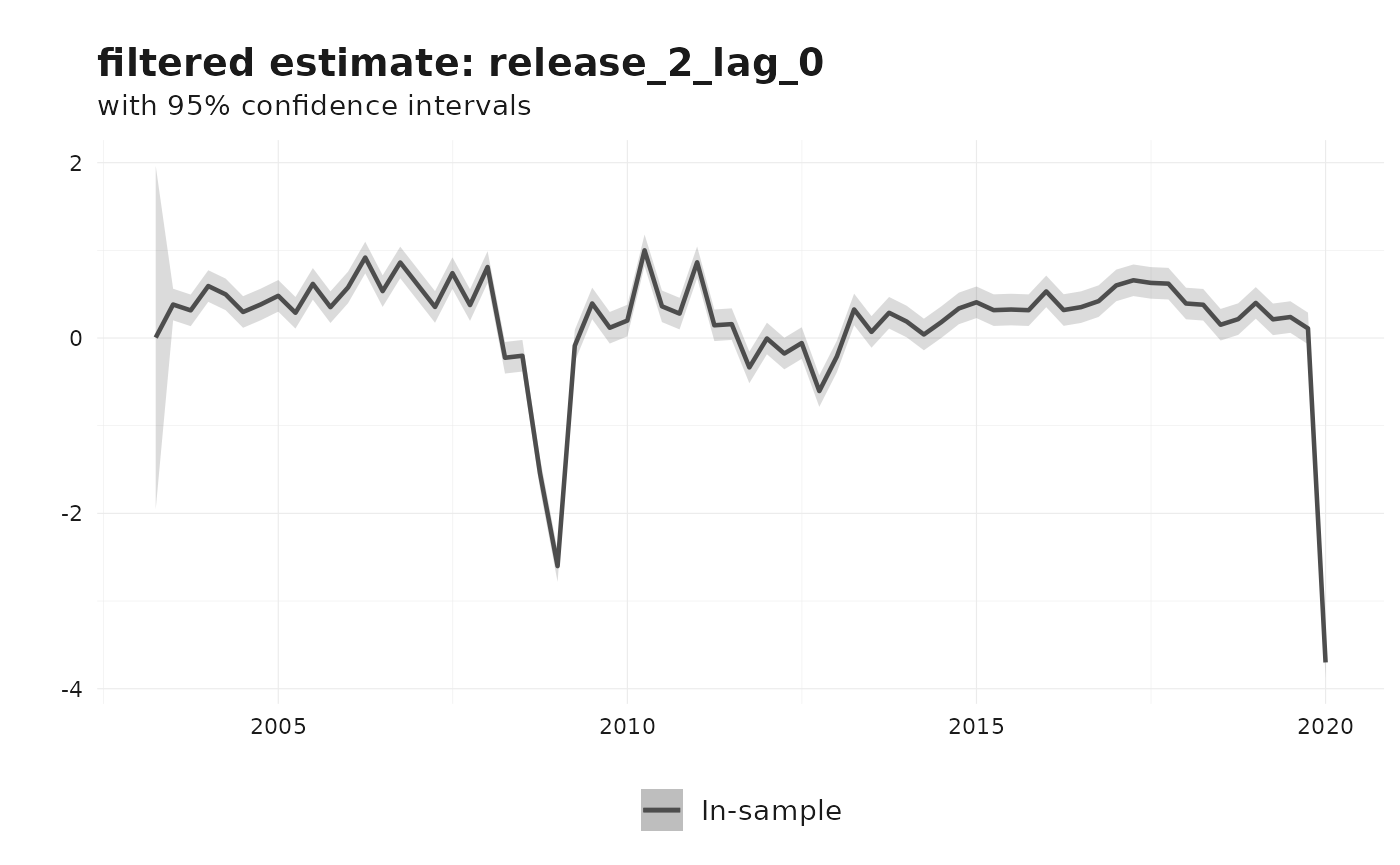

Other KK-family specifications

The same data can be estimated under the nested Howrey and Classical restrictions.

fit_howrey <- kk_nowcast(
  df = data_kk,
  e = e,
  model = "Howrey",
  method = "MLE"
)

fit_classical <- kk_nowcast(
  df = data_kk,
  e = e,
  model = "Classical",
  method = "MLE"
)

Those alternatives are useful when the unrestricted gain matrix of the full KK model is too parameter rich for the available sample.

Durbin, James, and Siem Jan Koopman. 2012. Time Series Analysis by State Space Methods: Second Edition. Oxford University Press. https://doi.org/10.1093/acprof:oso/9780199641178.001.0001.

Howrey, E. Philip. 1978. “The Use of Preliminary Data in Econometric Forecasting.” The Review of Economics and Statistics 60 (2): 193. https://doi.org/10.2307/1924972.