Nowcasting revisions using the Jacobs-Van Norden model

This vignette describes the Jacobs-Van Norden (JVN) revision model as implemented in reviser::jvn_nowcast(). The presentation follows the same Durbin-Koopman state-space notation used in the KK vignette: observations are linked to latent states through $Z$ , state dynamics through $T$ , and innovations through $R$ , $H$ , and $Q$ (Durbin and Koopman 2012).

The key idea of the JVN framework is that revision errors are not treated as a single residual. Instead, they are decomposed into news and noise. News corresponds to genuinely new information incorporated by later releases, whereas noise corresponds to transitory measurement error that is corrected in subsequent vintages (Jacobs and Van Norden 2011).

Revision decomposition

Let $l$ denote the number of vintages used in the model and let $y_t^{t+j}$ be the estimate for reference period $t$ available in vintage $t+j$ . Stack the vintages into

$y_t = \begin{bmatrix} y_t^{t+1} \\ y_t^{t+2} \\ \vdots \\ y_t^{t+l} \end{bmatrix}.$

Let $\tilde y_t$ denote the latent “true” value and let $\iota_l$ be an $l \times 1$ vector of ones. The JVN decomposition is

$y_t = \iota_l \tilde y_t + \nu_t + \zeta_t,$

where $\nu_t$ is the news component and $\zeta_t$ is the noise component.

$\nu_t$ captures information that was unavailable when early releases were produced and is therefore rationally incorporated later.
$\zeta_t$ captures transitory measurement error that is eventually revised away.

This decomposition is the main attraction of the JVN model: it separates revisions that reflect learning about the economy from revisions that reflect mistakes in earlier measurement.

Durbin-Koopman state-space form

In the notation of Durbin and Koopman (2012), the generic state-space model is

$y_t = Z \alpha_t + \varepsilon_t, \qquad \varepsilon_t \sim N(0, H),$

$\alpha_{t+1} = T \alpha_t + R \eta_t, \qquad \eta_t \sim N(0, Q).$

The current reviser implementation sets $H = 0$ , so all uncertainty enters through the transition equation. It also fixes $Q = I$ and places the scale parameters directly in the shock-loading matrix $R$ .

The `reviser` implementation

jvn_nowcast() implements a restricted but practical version of the JVN model. The latent true value follows an AR( $p$ ) process, and the user may include a news block, a noise block, or both. Optional spillovers are implemented as diagonal persistence terms in the selected measurement-error blocks.

When both news and noise are included, the state vector is

$\alpha_t = \begin{bmatrix} \tilde y_t \\ \tilde y_{t-1} \\ \vdots \\ \tilde y_{t-p+1} \\ \nu_t \\ \zeta_t \end{bmatrix},$

where $\nu_t$ and $\zeta_t$ are both $l \times 1$ vectors.

Measurement equation

With $l$ vintages and an AR( $p$ ) latent process, the observation matrix is

$Z = \begin{bmatrix} \iota_l & 0_{l \times (p - 1)} & I_l & I_l \end{bmatrix},$

so the observation equation is

$y_t = Z \alpha_t.$

If only news or only noise is included, the corresponding block is simply omitted from $Z$ .

Transition equation

The true-value block follows the companion-form AR( $p$ ) transition

$\Phi = \begin{bmatrix} \rho_1 & \rho_2 & \cdots & \rho_p \\ 1 & 0 & \cdots & 0 \\ 0 & 1 & \ddots & \vdots \\ \vdots & \vdots & \ddots & 0 \end{bmatrix}.$

The full transition matrix can therefore be written compactly as

$T = \begin{bmatrix} \Phi & 0 & 0 \\ 0 & T_{\nu} & 0 \\ 0 & 0 & T_{\zeta} \end{bmatrix},$

where $T_{\nu}$ and $T_{\zeta}$ are diagonal spillover blocks when spillovers are enabled and zero matrices otherwise.

Shock-loading matrix

The implementation uses $Q = I$ and places the innovation standard deviations inside $R$ .

The first structural shock loads on the latent true value with coefficient $\sigma_e$ .
The news shocks load negatively on the true value and positively on the news states in the upper-triangular pattern implied by jvn_update_matrices(). This enforces the idea that later vintages embed information unavailable to earlier vintages.
The noise shocks load independently on the corresponding noise states with coefficients $\sigma_{\zeta,1}, \dots, \sigma_{\zeta,l}$ .

This is the main implementation detail that differs from writing every variance parameter inside $Q$ : in reviser, $Q$ is fixed and $R$ carries the scale parameters.

Nested JVN specifications

The function covers the empirically relevant subclasses discussed by Jacobs and Van Norden (2011).

include_news = TRUE, include_noise = FALSE: pure news model
include_news = FALSE, include_noise = TRUE: pure noise model
include_news = TRUE, include_noise = TRUE: combined news-noise model
include_spillovers = TRUE: diagonal persistence in the selected measurement-error block(s)

Because these are nested specifications, information criteria are often useful for comparing them, although standard boundary-value caveats still apply.

Example: Euro Area GDP revisions

We illustrate the workflow with four vintages of Euro Area GDP growth from reviser::gdp.

library(reviser)
library(dplyr)
library(tidyr)
library(tsbox)
library(ggplot2)

gdp_growth <- reviser::gdp |>
  tsbox::ts_pc() |>
  dplyr::filter(
    id == "EA",
    time >= min(pub_date),
    time <= as.Date("2020-01-01")
  ) |>
  tidyr::drop_na()

df <- get_nth_release(gdp_growth, n = 0:3)
df
#> # Vintages data (release format):
#> # Format:                         long
#> # Time periods:                   70
#> # Releases:                       4
#> # IDs:                            1
#>    time       pub_date      value id    release  
#>    <date>     <date>        <dbl> <chr> <chr>    
#>  1 2002-10-01 2003-01-01  0.169   EA    release_0
#>  2 2002-10-01 2003-04-01  0.124   EA    release_1
#>  3 2002-10-01 2003-07-01  0.105   EA    release_2
#>  4 2002-10-01 2003-10-01  0.0577  EA    release_3
#>  5 2003-01-01 2003-04-01  0.0149  EA    release_0
#>  6 2003-01-01 2003-07-01 -0.0133  EA    release_1
#>  7 2003-01-01 2003-10-01 -0.0558  EA    release_2
#>  8 2003-01-01 2004-01-01 -0.00601 EA    release_3
#>  9 2003-04-01 2003-07-01  0.00503 EA    release_0
#> 10 2003-04-01 2003-10-01 -0.0616  EA    release_1
#> # ℹ 270 more rows

The resulting data frame has one row per reference period and one column per release, which is the format expected by jvn_nowcast().

fit_jvn <- load_or_build_vignette_result(
  "nowcasting-revisions-jvn-fit.rds",
  function() {
    jvn_nowcast(
      df = df,
      e = 4,
      ar_order = 2,
      h = 0,
      include_news = TRUE,
      include_noise = TRUE,
      include_spillovers = TRUE,
      spillover_news = TRUE,
      spillover_noise = TRUE,
      method = "MLE",
      standardize = FALSE,
      solver_options = list(
        method = "L-BFGS-B",
        maxiter = 100,
        se_method = "hessian"
      )
    )
  }
)

summary(fit_jvn)
#> 
#> === Jacobs-Van Norden Model ===
#> 
#> Convergence: Failed 
#> Log-likelihood: 265.89 
#> AIC: -493.78 
#> BIC: -451.06 
#> 
#> Parameter Estimates:
#>     Parameter Estimate Std.Error
#>         rho_1    0.378     0.362
#>         rho_2    0.179     0.122
#>       sigma_e    0.485     0.128
#>    sigma_nu_1    0.001     0.039
#>    sigma_nu_2    0.047     0.004
#>    sigma_nu_3    0.007     0.058
#>    sigma_nu_4    1.088     1.591
#>  sigma_zeta_1    0.046     0.012
#>  sigma_zeta_2    0.003     0.006
#>  sigma_zeta_3    0.008     0.000
#>  sigma_zeta_4    0.039     0.010
#>        T_nu_1    0.150     0.078
#>        T_nu_2    0.107     0.087
#>        T_nu_3    0.094     0.097
#>        T_nu_4    0.086     0.105
#>      T_zeta_1   -0.185     0.423
#>      T_zeta_2   -0.900     0.000
#>      T_zeta_3   -0.634     0.111
#>      T_zeta_4    0.146     0.113

The parameter table contains the AR coefficients, the latent-process innovation scale $\sigma_e$ , the news and noise innovation scales, and, when selected, the diagonal spillover persistence parameters.

fit_jvn$params
#>       Parameter     Estimate   Std.Error
#> 1         rho_1  0.378378980 0.361677538
#> 2         rho_2  0.179154350 0.121871675
#> 3       sigma_e  0.485087544 0.127563589
#> 4    sigma_nu_1  0.001000000 0.039456621
#> 5    sigma_nu_2  0.047177947 0.003942688
#> 6    sigma_nu_3  0.006547902 0.057869870
#> 7    sigma_nu_4  1.087596777 1.590627455
#> 8  sigma_zeta_1  0.045978422 0.012375310
#> 9  sigma_zeta_2  0.002968998 0.005930814
#> 10 sigma_zeta_3  0.008115144 0.000000000
#> 11 sigma_zeta_4  0.038936158 0.009748625
#> 12       T_nu_1  0.150090145 0.078021418
#> 13       T_nu_2  0.106883324 0.087466061
#> 14       T_nu_3  0.093954764 0.096747489
#> 15       T_nu_4  0.085946442 0.105141486
#> 16     T_zeta_1 -0.185315823 0.423426245
#> 17     T_zeta_2 -0.900000000 0.000000000
#> 18     T_zeta_3 -0.633719067 0.111249751
#> 19     T_zeta_4  0.145519819 0.113131616

The state named true_lag_0 is the current latent true value.

fit_jvn$states |>
  dplyr::filter(
    state == "true_lag_0",
    filter == "smoothed"
  ) |>
  dplyr::slice_tail(n = 8)
#> # A tibble: 8 × 7
#>   time       state      estimate  lower  upper filter   sample   
#>   <date>     <chr>         <dbl>  <dbl>  <dbl> <chr>    <chr>    
#> 1 2018-04-01 true_lag_0    0.406 -0.902  1.71  smoothed in_sample
#> 2 2018-07-01 true_lag_0    0.720 -0.589  2.03  smoothed in_sample
#> 3 2018-10-01 true_lag_0    0.746 -0.563  2.05  smoothed in_sample
#> 4 2019-01-01 true_lag_0    0.155 -1.15   1.46  smoothed in_sample
#> 5 2019-04-01 true_lag_0    1.04  -0.273  2.34  smoothed in_sample
#> 6 2019-07-01 true_lag_0   -1.11  -2.42   0.201 smoothed in_sample
#> 7 2019-10-01 true_lag_0   -3.20  -4.56  -1.84  smoothed in_sample
#> 8 2020-01-01 true_lag_0   -4.04  -6.18  -1.90  smoothed in_sample

The default plot method shows the filtered estimate of the latent true value.

plot(fit_jvn)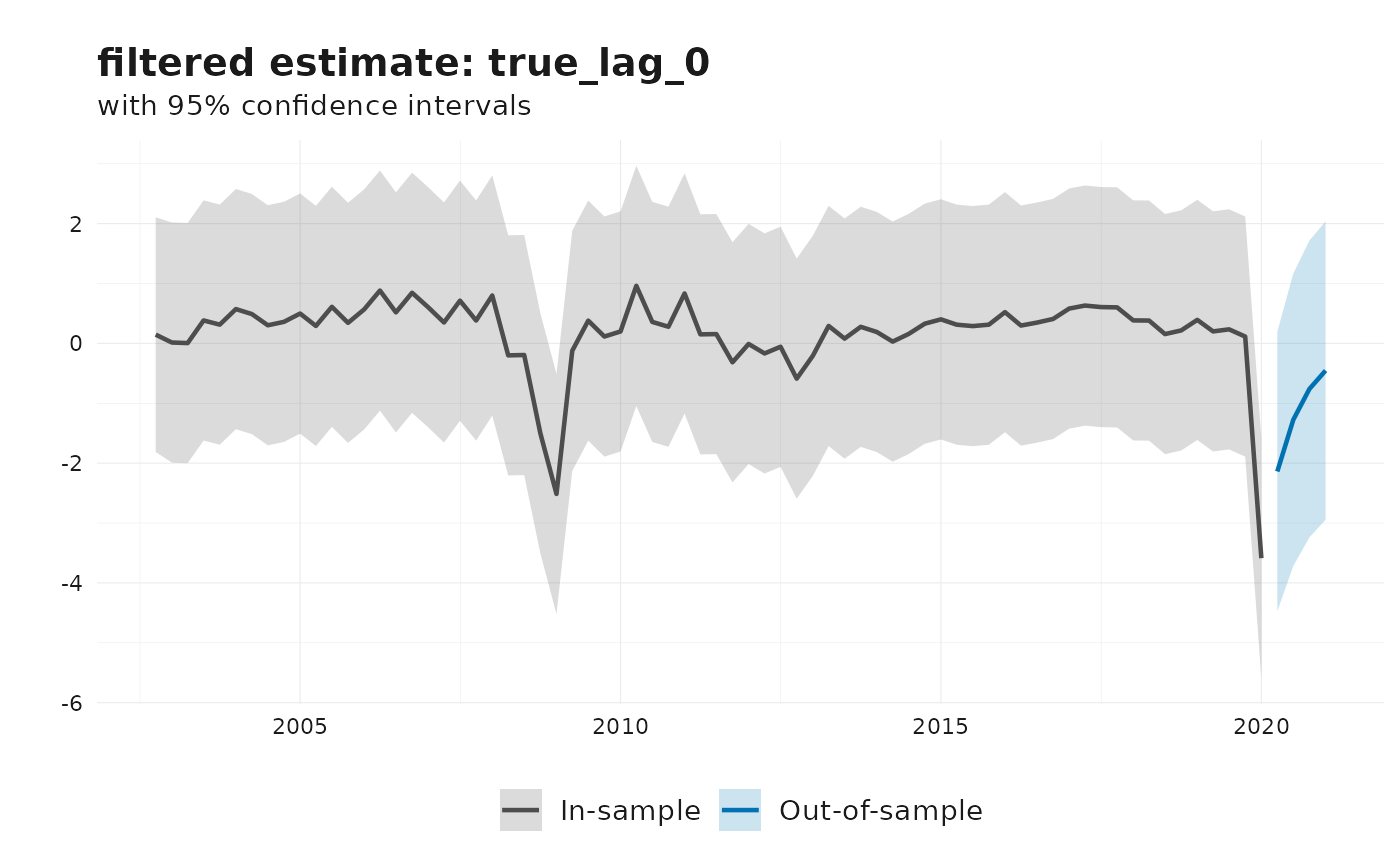

We can also inspect the smoothed news and noise states directly.

fit_jvn$states |>
  dplyr::filter(
    filter == "smoothed",
    grepl("news|noise", state)
  ) |>
  ggplot(aes(x = time, y = estimate, color = state)) +
  geom_line() +
  labs(
    title = "Smoothed news and noise states",
    x = NULL,
    y = "State estimate"
  ) +
  theme_minimal()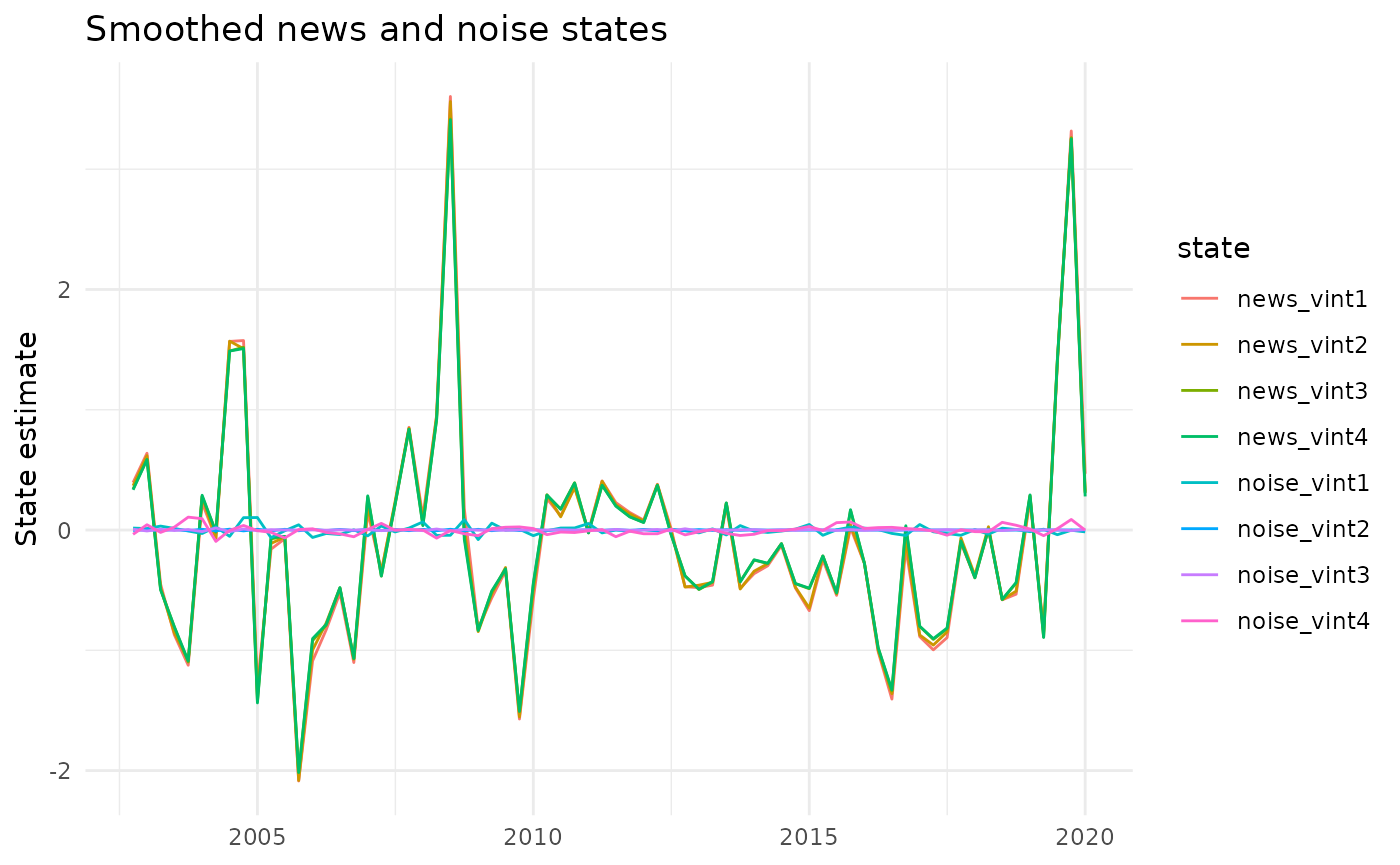

Other JVN specifications

Pure-news and pure-noise variants are obtained by switching off the unwanted measurement-error block.

fit_news <- jvn_nowcast(
  df = df,
  e = 4,
  ar_order = 2,
  include_news = TRUE,
  include_noise = FALSE,
  include_spillovers = FALSE
)

fit_noise <- jvn_nowcast(
  df = df,
  e = 4,
  ar_order = 2,
  include_news = FALSE,
  include_noise = TRUE,
  include_spillovers = FALSE
)

If desired, the data can be approximately standardized before estimation using standardize = TRUE. In that case, scaling metadata are returned in the scale element of the fitted object.

Durbin, James, and Siem Jan Koopman. 2012. Time Series Analysis by State Space Methods: Second Edition. Oxford University Press. https://doi.org/10.1093/acprof:oso/9780199641178.001.0001.

Jacobs, Jan P. A. M., and Simon Van Norden. 2011. “Modeling Data Revisions: Measurement Error and Dynamics of ‘True’ Values.” Journal of Econometrics 161 (2): 101–9. https://doi.org/10.1016/j.jeconom.2010.04.010.