Understanding Data Revisions

This vignette introduces the notation used in the literature and presents the revision triangle as a foundational structure for analyzing revisions. Then, it illustrates how to use the function get_revisions() to extract revisions from time series data. Finally, we illustrate with a detailed example how data revisions can be extracted and illustrated.

Introduction: Why do data revisions occur?

Economic and statistical data, in particular time series data, are frequently revised after their initial publication. These revisions occur due to a variety of reasons, including methodological updates, newly available data, and technical adjustments. Understanding why revisions happen is crucial for properly interpreting economic indicators and assessing data reliability.

Revisions can be classified into several key categories:

Type of Revision	Cause
Content Revisions	Updates due to the incorporation of newly available information
Base Data Revisions	Adjustments when new benchmark data is released
Benchmark Revisions	Structural changes in methodology
Minor Changes in Estimation Methods	Continuous refinements in models
Technical Adjustments	Data corrections or econometric technique updates
Economic Events & Shocks	Large-scale disruptions necessitating revisions
Technological Advances	Integration of new data sources or methods

Incorporation of newly available or updated data

Initial estimates of economic indicators are often based on partial or preliminary data. As more comprehensive information becomes available, statistical agencies revise their figures to reflect the most accurate representation of economic activity. This is common for GDP estimates, labor statistics, and to a lesser extent also inflation measures. Many statistical agencies use interpolation and extrapolation techniques to estimate quarterly indicators based on incomplete information. When new input data becomes available, past estimates are revised to align with the improved dataset (Sax and Steiner 2013).

Example: The U.S. Bureau of Economic Analysis (BEA) revises GDP estimates multiple times as more data becomes available.

Base data revisions

Annual macroeconomic data, such as national accounts and GDP, are often revised when new yearly aggregates are released. Statistical offices typically revise figures for the most recent two to three years, while older data remains unchanged unless there is a major methodological update.

Example: The Swiss Federal Statistical Office (SFSO) revises past two years of annual GDP each August.

Benchmark revisions (methodological changes)

Concepts and methodologies used in national accounts evolve over time to comply with new international standards and improve accuracy. Benchmark revisions introduce major changes that may affect the entire historical time series.

Examples of benchmark revisions in Swiss GDP measurement:

Year	Major Change
2004	Adjustments to European System of Accounts (ESA 1995)
2009	Shift from direct to indirect seasonal adjustment
2014	Transition to ESA 2010 standards

These revisions can significantly alter growth rates, levels, and historical trends.

Minor changes in estimation methods

Even when large-scale benchmark revisions do not occur, statistical agencies continuously refine their estimation methods:

Adjustments to seasonal adjustment techniques.
Replacing outdated indicators with new ones.
Improving econometric models for nowcasting and forecasting.

Example: Changes in how consumer confidence indexes are incorporated into GDP forecasts.

Technical adjustments & error corrections

Revisions can occur due to simple technical adjustments, including:

Correction of data entry errors.
Adjustments due to missing or late-reported data.
Revisions in survey weighting methods.

Example: The Bureau of Labor Statistics (BLS) revises employment data as late reports from firms are incorporated.

Economic events & shocks

Unforeseen economic events often require large-scale revisions due to structural breaks in economic activity.

Examples:

COVID-19 pandemic: GDP estimates revised significantly as lockdowns disrupted economic data collection.
Financial crises: Banking sector collapses lead to re-evaluation of past financial statistics.

These events create higher-than-normal uncertainty, necessitating frequent revisions.

Technological advances in data collection

The adoption of big data, machine learning, and AI in economic statistics has introduced new ways to process and analyze data. These technological advances can lead to revisions as agencies shift to more sophisticated data integration methods.

Example: Nowcasting models using high-frequency data (e.g., credit card transactions) influence revisions in real-time GDP estimates.

Some mathematical notation

The notation follows standard conventions in the literature:

Superscripts (vintage) refer to when the estimate was available.
Subscripts (time) refer to when the observation was recorded.

For example: \( y_1^t \) is the estimate available at time \( t \) of the value of variable \( y \) at time 1.

In general: \( y_j^t \) represents the estimate of \( y \) at time \( j \), released in vintage \( t \).

Revisions are often studied in the form of a revision triangle, where:

\[ Y = \begin{bmatrix} y_1^1 & & y_1^{t-l} & & y_1^t \\ & \ddots & \vdots & \vdots & \vdots \\ & & y_{t-l}^{t-l} & \cdots & y_{t-l}^t \\ & & & \ddots & \vdots \\ & & & & y_t^t \\ \end{bmatrix} \]

where each row corresponds to a specific time period and each column corresponds to a successive release of the data. As we move rightward, we see later vintages (updated data releases).As we move downward, we observe later time periods.

Extracting revisions with reviser

Now that we understand why revisions occur, the next step is to quantify and analyze them. In economic statistics, real-time data consists of multiple vintages of observations, where each vintage represents a successive release of the data. These vintages are stored in a revision triangle, also known as a real-time data matrix, where:

Rows represent the time periods of the original observations.
Columns represent successive vintages (or releases) of the data.

The `get_revisions()` function

Once the data under scrutiny is formatted along the lines illustrated in the introduction to reviser, i.e., in long tidy format the data tibble consists of:

time, the time period
pub_date and/or release, the publication date or release number
value, the reported value.
id, an optional column to distinguish between different series

then we can extract the revisions inherent in our time series vintages with the function get_revisions(). The function allows users to compute revisions by comparing different vintages of a time series dataset. It supports three primary methods:

Fixed Reference Date (ref_date): Computes revisions relative to a fixed publication date.
Nth Release (nth_release): Compares revisions to the nth release of a data point.
Interval Lag (interval): Measures changes between vintages published a fixed number of periods apart.

Example usage

Once we have formatted our dataset in the appropriate long tidy format, we can apply the get_revisions() function to analyze revisions using different methods. Below are some practical examples using GDP revision data.

Example 1: Revisions Using an Interval

The most common use case is to analyze how reported values evolve over time. By setting interval = 1, we compute revisions between consecutive releases:

library(dplyr)
#> 
#> Attaching package: 'dplyr'
#> The following objects are masked from 'package:stats':
#> 
#>     filter, lag
#> The following objects are masked from 'package:base':
#> 
#>     intersect, setdiff, setequal, union
library(reviser)
library(tsbox)

# Example dataset
gdp <- reviser::gdp %>%
  ts_pc() %>%
  na.omit()

revisions_interval <- get_revisions(gdp, interval = 1)

# Preview results
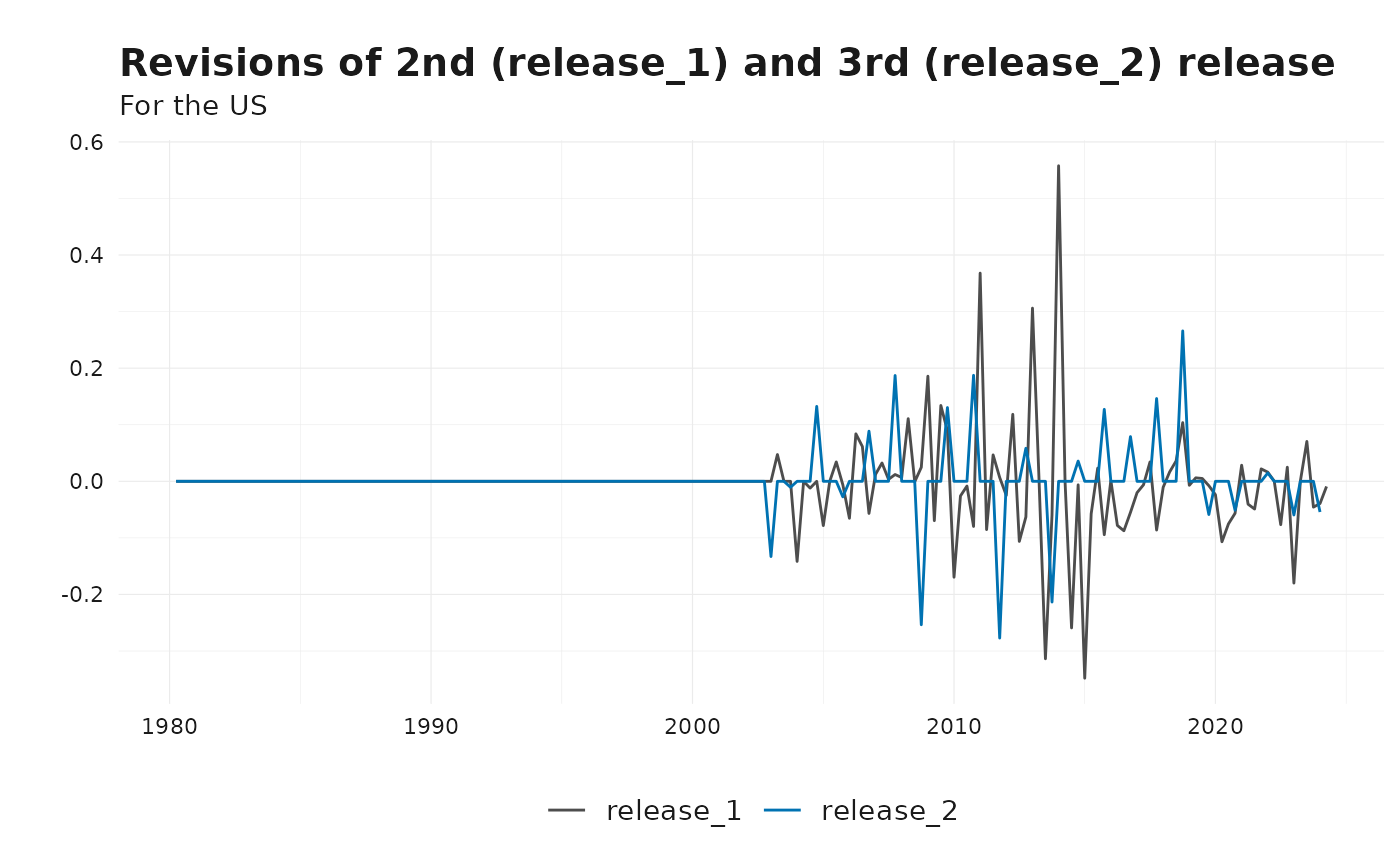
# How do the 2nd and 3rd release revise compared to previous quarter?
plot_vintages(
  revisions_interval %>% 
    filter(id == "US") %>%
    get_nth_release(1:2),
  dim_col = "release",
  title = "Revisions of 2nd (release_1) and 3rd (release_2) release",
  subtitle = "For the US"
)


# Revisions of the latest release
plot_vintages(
  revisions_interval %>% get_latest_release(),
  dim_col = "id",
  title = "Revisions of the latest release",
  subtitle = "For several countries"
)
#> Warning: Removed 4 rows containing missing values or values outside the scale range
#> (`geom_line()`).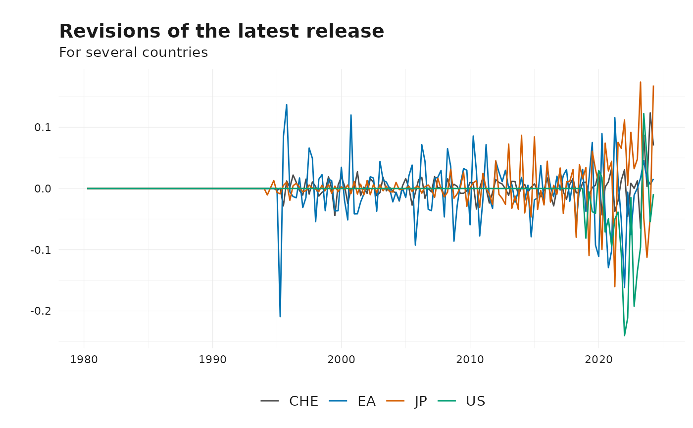

This helps identify patterns in how the data is revised over time, whether revisions are systematic or random, and their magnitude.

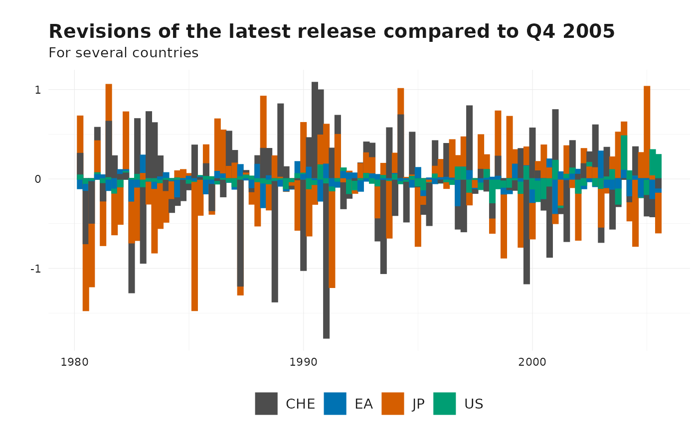
Example 2: Revisions Relative to a Fixed Reference Date

To compare all reported values against a fixed publication date, use the ref_date argument. This is useful when benchmarking against an initial estimate:


revisions_date <- get_revisions(gdp, ref_date = as.Date("2005-10-01"))

# Preview results
# Revisions of the latest release
plot_vintages(
  revisions_date %>% get_latest_release(),
  dim_col = "id",
  title = "Revisions of the latest release compared to Q4 2005",
  subtitle = "For several countries",
  type="bar"
)

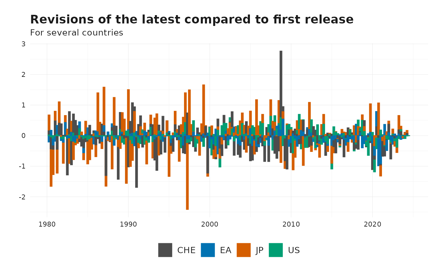
Example 3: Revisions to the Nth Release

Instead of comparing consecutive releases, we can compare each data point against its nth release. For example, if we want to evaluate revisions between the first and last releases:

revisions_nth <- get_revisions(gdp, nth_release = 0)

# Preview results
# Revisions of the latest release
plot_vintages(
  revisions_nth %>% get_latest_release(),
  dim_col = "id",
  title = "Revisions of the latest compared to first release",
  subtitle = "For several countries",
  type="bar"
)

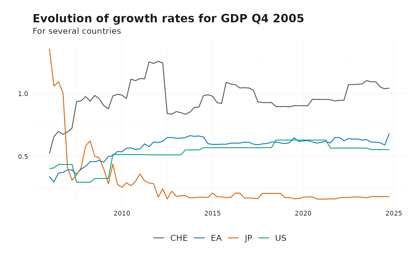
Example 4: How does the growth rate of GDP change over time?


growthrates_q405 <- get_releases_by_date(gdp, as.Date("2005-10-01"))
  

# Preview results
plot_vintages(
  growthrates_q405,
  dim_col = "id",
  time_col = "pub_date",
  title = "Evolution of growth rates for GDP Q4 2005",
  subtitle = "For several countries",
  type="line"
)

References

Sax, Christoph, and Peter Steiner. 2013. “Temporal Disaggregation of Time Series.” R Journal 5 (2).